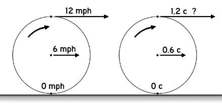
When a wheel rolls without slipping along a pavement, the rim speed of its contact point with the pavement is zero in the pavement reference frame, while the rim speed at the top of the wheel is twice the speed of the wheel itself. This presents a paradox when the wheel rolls at relativistic speeds, where the rim speed at the top might exceed c, the speed of light.
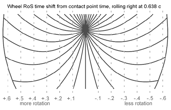
The paradox is currently resolved using relativistic addition of velocities, relativity of simultaneity (hereinafter RoS), or a combination of the two. The wheel experiences Lorentz contraction in the direction of motion, yielding a tall ellipse in the pavement frame. Sections of the rim at the top of the wheel are contracted, while sections at the bottom are expanded. This is often illustrated by an elliptical spoked wheel, with spokes curving upward as RoS varies their amount of rotation. Shown here at 0.638 c.
With increasing horizontal distance from the pavement contact point normal (the vertical line through the center of the wheel), time in the leading half of the wheel gets progressively earlier, and because the rotation in the forward section is downward, the spokes show progressively less rotation, curving them upward. In the trailing half of the wheel, time goes progressively later, resulting in spokes showing progressively more rotation, which also curves them upward.
This solution to the paradox is satisfactory to all wheel speeds short of c, keeping the pavement frame rim speed at the top of the wheel below c.
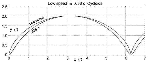
However, this solution does not address the pavement frame path of a point on the rim of the wheel as the wheel rolls along. A rim point describes an arched path between pavement contacts called a cycloid.

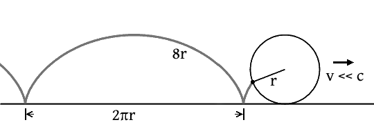
Conventional geometry has the length of a cycloid at 8 r. The rollout length of a non-slipping wheel is 2 π r. The simple ratio of these lengths means the speed of the rolling wheel in the pavement frame must be less than 0.785 c, even if the cycloid path were traversed entirely at the speed of light.
The cycloid path however must start and end at the contact points with a speed of zero in the pavement frame. This further reduces the maximum speed allowable for the wheel.
It is anticipated that Lorentz contraction of the wheel and the RoS shift of the point position will alter the shape of the cycloid, narrowing it somewhat in its upper section, which in turn will widen it around the contact point. This generates an inflection that precludes using a common method of determining the cycloid point speed by vector addition, thus numerical methods are used.
The algorithm pseudocode is included as an appendix. It is annotated with explanatory comments.
The x and y coordinates of a point on the cycloid are calculated separately.
x = r(t - sin t)
y = r(1 - cos t)
where t is the contact point of a circle rolling on the x axis.
The position obtained is adjusted for RoS, then Lorentz contracted.
Adjusting for RoS alters the distance from the contact point normal, which changes the amount of adjustment required. Depending on the quadrant (loosely defined) and speed of the wheel, the change may be either positive or negative, so an iterative approach is taken.
Generated data points are equally spaced in pavement frame time, so the distance between them translates directly to speed between points. The algorithm tracks the maximum speed obtained. Due to the nature of π, the top of the cycloid cannot be hit exactly, and only the initial contact point is exact.
Vertical axis expanded.
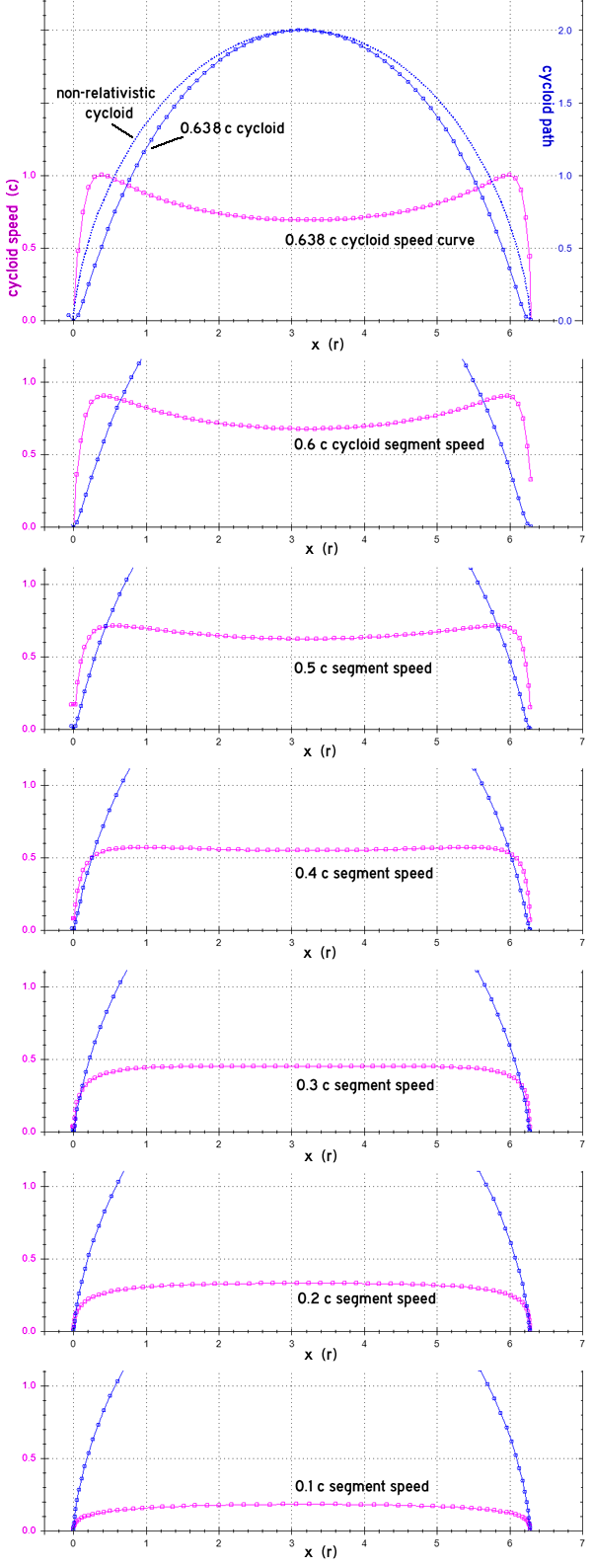
1. There is an upper speed limit of 0.638... c for a wheel rolling on a pavement without slipping. Greater wheel speeds result in points on the cycloid exceeding c.
2. The body of the cycloid becomes slightly narrower as wheel speed increases. The contact point path opens from a vertical 'bounce' to more of a 'skip.'
3. A run with Lorentz contraction disabled shows that the majority of the cycloid alteration is due to RoS.
4. The speed plots show that as wheel speed increases, the maximum speed location shifts from the top center of the arch, splitting off to each side, with the speed curve sagging as the generating point goes over the top of the wheel.
5. The pavement frame is a ubiquitous example of an inertial frame instantaneously co-moving with the wheel rim. The speed limitation has implications for other situations in relativistic rotation, as such frames may be established at any radius and direction for any object in rotation.